Reading and Writing Data

Code and text for Quiz 4.

1. Load the R packages we will use.

library(tidyverse)
library(here)
library(janitor)
library(skimr)

2. Download \(CO_2\) emissions per capita from Our World in Data into the directory for this post.

3. Assign the location of the file to file.csv. The data should be in the same directory as this file.

• Read the data into R and assign it to emissions

file_csv <- here("_posts",
                 "2021-02-16-reading-and-writing-data",
                 "co-emissions-per-capita.csv")
emissions <- read_csv(file_csv)

4. Show the first 10 rows (observations of) emissions

emissions

# A tibble: 22,383 x 4
   Entity      Code   Year `Per capita CO2 emissions`
   <chr>       <chr> <dbl>                      <dbl>
 1 Afghanistan AFG    1949                    0.00191
 2 Afghanistan AFG    1950                    0.0109 
 3 Afghanistan AFG    1951                    0.0117 
 4 Afghanistan AFG    1952                    0.0115 
 5 Afghanistan AFG    1953                    0.0132 
 6 Afghanistan AFG    1954                    0.0130 
 7 Afghanistan AFG    1955                    0.0186 
 8 Afghanistan AFG    1956                    0.0218 
 9 Afghanistan AFG    1957                    0.0343 
10 Afghanistan AFG    1958                    0.0380 
# ... with 22,373 more rows

5. Start with emissions data THEN

   • use clean names from the janitor package to make the names easier to work with

   • assign the output to tidy_emissions

   • show the first 10 rows of tidy_emissions

tidy_emissions <- emissions %>%
  clean_names()
tidy_emissions

# A tibble: 22,383 x 4
   entity      code   year per_capita_co2_emissions
   <chr>       <chr> <dbl>                    <dbl>
 1 Afghanistan AFG    1949                  0.00191
 2 Afghanistan AFG    1950                  0.0109 
 3 Afghanistan AFG    1951                  0.0117 
 4 Afghanistan AFG    1952                  0.0115 
 5 Afghanistan AFG    1953                  0.0132 
 6 Afghanistan AFG    1954                  0.0130 
 7 Afghanistan AFG    1955                  0.0186 
 8 Afghanistan AFG    1956                  0.0218 
 9 Afghanistan AFG    1957                  0.0343 
10 Afghanistan AFG    1958                  0.0380 
# ... with 22,373 more rows

6. Start with the tidy_emissions THEN

   • use filter to extract rows with year==1985 THEN

   • use skim to calculate the descriptive statistics

tidy_emissions %>%
  filter(year==1985) %>%
  skim()

Table 1: Data summary

Name	Piped data
Number of rows	209
Number of columns	4
_______________________
Column type frequency:
character	2
numeric	2
________________________
Group variables	None

Variable type: character

skim_variable	n_missing	complete_rate	min	max	empty	n_unique	whitespace
entity	0	1.00	4	32	0	209	0
code	12	0.94	3	8	0	197	0

Variable type: numeric

skim_variable	n_missing	complete_rate	mean	sd	p0	p25	p50	p75	p100	hist
year	0	1	1985.00	0.00	1985.00	1985.00	1985.00	1985.00	1985.00	▁▁▇▁▁
per_capita_co2_emissions	0	1	5.53	8.94	0.04	0.51	2.65	7.62	83.83	▇▁▁▁▁

7. 12 observations have a missing code. How are these observations different?

   • start with tidy_emissions then extract rows with year == 1985 and are missing a code

tidy_emissions %>%
  filter(year==1985, is.na(code))

# A tibble: 12 x 4
   entity                     code   year per_capita_co2_emissions
   <chr>                      <chr> <dbl>                    <dbl>
 1 Africa                     <NA>   1985                     1.23
 2 Asia                       <NA>   1985                     1.81
 3 Asia (excl. China & India) <NA>   1985                     2.76
 4 EU-27                      <NA>   1985                     9.19
 5 EU-28                      <NA>   1985                     9.28
 6 Europe                     <NA>   1985                    10.9 
 7 Europe (excl. EU-27)       <NA>   1985                    13.3 
 8 Europe (excl. EU-28)       <NA>   1985                    14.1 
 9 North America              <NA>   1985                    13.2 
10 North America (excl. USA)  <NA>   1985                     5.01
11 Oceania                    <NA>   1985                    10.8 
12 South America              <NA>   1985                     1.87

Entities that are not countries do not have country codes.

8. Start with tidy_emissions THEN

   • use filter to extract rows with year==1985 and without missing codes THEN

   • use select to drop the year variable THEN

   • use rename to change the variable entity to country

   • assign the output to emissions_1985

emissions_1985 <- tidy_emissions %>%
  filter(year==1985, !is.na(code)) %>%
  select(-year) %>%
  rename(country=entity)

9. Which 15 countries have the highest per_capita_co2_emissions?

   • start with emissions_1985 THEN

   • use slice_max to extract the 15 rows with the highest values

   • assign the output to max_15_emitters

max_15_emitters <- emissions_1985 %>%
  slice_max(per_capita_co2_emissions, n=15)

10. Which 15 countries have the lowest per_capita_co2_emissions?

    • start with emissions_1985 THEN

    • use slice_min to extract the 15 rows with the lowest values

    • assign the output to min_15_emitters

min_15_emitters <- emissions_1985 %>%
  slice_min(per_capita_co2_emissions, n=15)

11. Use bind_rows to bind together the max_15_emitters and min_15_emitters

    • assign the output to max_min_15

max_min_15 <- bind_rows(max_15_emitters, min_15_emitters)

12. Export max_min_15 to 3 file formats

max_min_15 %>% write_csv("max_min_15.csv") # comma-separated values
max_min_15 %>% write_tsv("max_min_15.tsv") # tab separated
max_min_15 %>% write_delim("max_min_15.psv", delim = "|") #pipe-separated

13. Read the 3 file formats into R

max_min_15_csv <- read_csv("max_min_15.csv") # comma-separated values
max_min_15_tsv <- read_tsv("max_min_15.tsv") # tab separated
max_min_15_psv <- read_delim("max_min_15.psv", delim = "|") #pipe-separated

14. Use setdiff to check for any differences among max_min_15_csv, max_min_15_tsv and max_min_15_psv

setdiff(max_min_15_csv, max_min_15_tsv, max_min_15_psv)

# A tibble: 0 x 3
# ... with 3 variables: country <chr>, code <chr>,
#   per_capita_co2_emissions <dbl>

Are there any differences?

15. Reorder country in max_min_15 for plotting and assign to max_min_15_plot_data

    • start with emissions_1985 THEN

    • use mutate to reorder country according to per_capital_co2_emissions

max_min_15_plot_data <- max_min_15 %>%
  mutate(country=reorder(country, per_capita_co2_emissions))

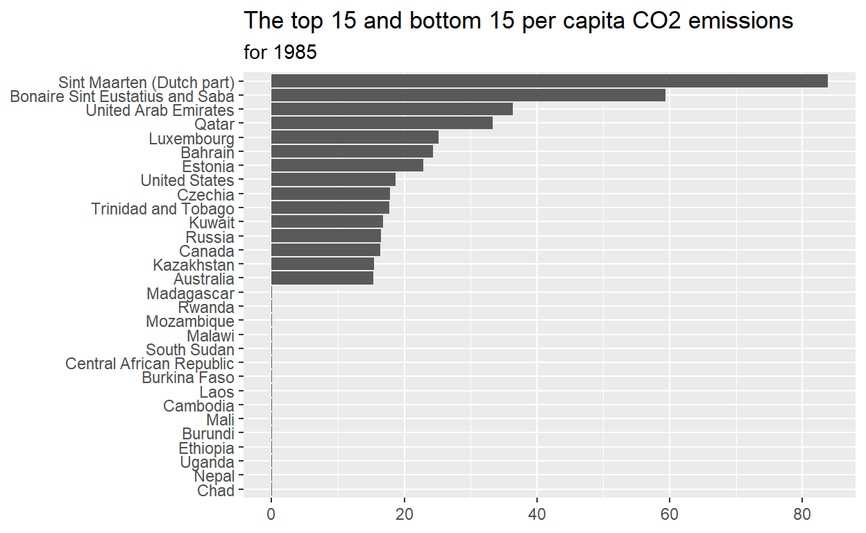
16. Plot max_min_15_plot_data

ggplot(data = max_min_15_plot_data ,
       mapping=aes(x=per_capita_co2_emissions, y=country))+
  geom_col()+
  labs(title="The top 15 and bottom 15 per capita CO2 emissions",
       subtitle = "for 1985",
       x=NULL,
       y=NULL)

17. Save the plot directory with this post

ggsave(filename = "preview.png",
       path=here("_posts", "2021-02-16-reading-and-writing-data"))

18. Add preview.png to yaml chunk at the top of this file

preview:preview.png